Cell transfer across ST slides of multiple time points
Multiple ST tissue sections obtained at different timepoints offer a valuable opportunity to gain a deeper understanding of cell transitions during organ development, such as mouse midbrain development and zebrafish embryogenesis. spaTrack can provide a novel strategy to infer cell tracing across multiple tissue sections based on an unbalanced and structured optimal transport algorithm by direct mapping cells among samples without integrating data. This approach is designed for cases where multiple sections containing the same cell types.In this tutorial, We use mouse midbrain ST data to demonstrate cell transfer across ST slides of multiple time points.
[1]:
import warnings
warnings.filterwarnings("ignore")
[2]:
import spaTrack as spt
import scanpy as sc
import pandas as pd
import matplotlib.pyplot as plt
sc.settings.verbosity = 0
plt.rcParams['figure.dpi'] = 200 #分辨率
1.Prepare ST data
Spatial transcriptmic data of mouse midbrain at E12.5,E14.5 and E16.5 time points were downloaded from published paper(Chen et al.2022, Cell). The example of expression tsv file and additional information file in this part can be download from Baidu Netdisk and Google Drive .We focused on progenitors cells including RGC(radial glia cells),NeuB(neuroblasts) and GlioB(glioblasts) to describe transfer relations among these progenitors cells.
[3]:
adata_all=sc.read('../../../../data/mouse.midbrain.three.time/mouse midbrain.three.time.point.ST.exp.tsv')
df_annot=pd.read_table('../../../../data/mouse.midbrain.three.time/meta.tsv',sep='\t',index_col=[0])
adata_all.obs=df_annot
adata_all.obs.index=list(df_annot.index)
adata_all.obsm['spatial']=adata_all.obs[['x','y']].values
adata_all.obs['CellID']=adata_all.obs.index
[4]:
adata_all.obs.head()
[4]:
| annotation | Time point | x | y | batch | CellID | |
|---|---|---|---|---|---|---|
| CELL.100034_1 | RGC | E12.5 | 2829.0 | -10000.0 | 0 | CELL.100034_1 |
| CELL.100795_1 | RGC | E12.5 | 2893.0 | -9946.5 | 0 | CELL.100795_1 |
| CELL.100841_1 | RGC | E12.5 | 2672.0 | -9944.0 | 0 | CELL.100841_1 |
| CELL.100867_1 | RGC | E12.5 | 2728.0 | -9943.0 | 0 | CELL.100867_1 |
| CELL.100880_1 | RGC | E12.5 | 2927.0 | -9939.0 | 0 | CELL.100880_1 |
[5]:
adata1_sub=adata_all[adata_all.obs['Time point']=='E12.5']
adata2_sub=adata_all[adata_all.obs['Time point']=='E14.5']
adata3_sub=adata_all[adata_all.obs['Time point']=='E16.5']
adata_all.uns['annotation_colors']=['#9A154C', '#F3754E', '#5B58A7']
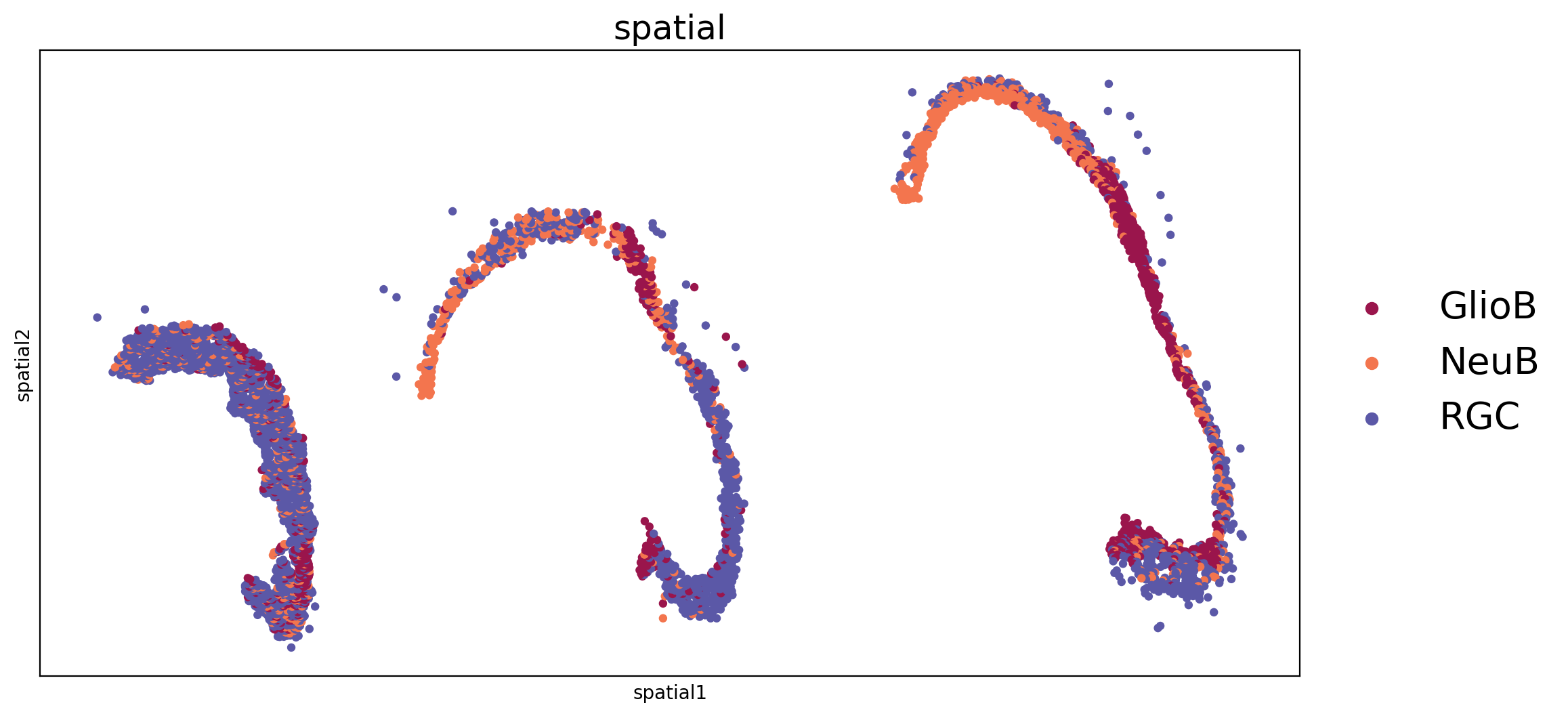
Visualzation of mouse midbrain ST data of three time points.
[6]:
fig, axs = plt.subplots(ncols=1, nrows=1, figsize=(12, 6))
sc.pl.embedding(adata_all, basis='spatial', color='annotation', size=50, legend_loc='right margin', legend_fontsize=20,ax=axs, legend_fontoutline=3, show=False, s=80)
axs.set_title('spatial',fontsize=18)
[6]:
Text(0.5, 1.0, 'spatial')
2.Calculate transition probability across sections
spaTrack infers cell tracing across multiple ST sections based on an unbalanced and structured optimal transport algorithm. We can calculate the transfer matrix between two ST sections using the spt.transfer_matrix function. Additionally, the transition probability between two sections can be calculated using spt.map_data. To obtain complete results across multiple sections, spt.generate_animate_input was used to integrate the transition probability results.
[7]:
pi12 = spt.transfer_matrix(adata1_sub,adata2_sub,epsilon=0.01,alpha=0.5)
pi23 = spt.transfer_matrix(adata2_sub,adata3_sub,epsilon=0.01,alpha=0.5)
We also can obtain the result containing cell transition probability among three ST sections.
[8]:
pi_matrix_coord = spt.generate_animate_input(pi_list=[pi12,pi23], adata_list=[adata1_sub,adata2_sub,adata3_sub],time ='Time point',annotation='annotation')
# pi_matrix_coord=pi_matrix_coord.loc[(pi_matrix_coord['pi_value1']> value1) & (pi_matrix_coord['pi_value1']> value2) ]
pi_matrix_coord.to_csv("./cell.transfer.csv")
[9]:
pi_matrix_coord.head()
[9]:
| slice1 | slice2 | slice3 | slice1_annotation | slice2_annotation | slice3_annotation | slice1_x | slice2_x | slice3_x | slice1_y | slice2_y | slice3_y | k_line_12 | b_line_12 | k_line_23 | b_line_23 | pi_value1 | pi_value2 | |
|---|---|---|---|---|---|---|---|---|---|---|---|---|---|---|---|---|---|---|
| 0 | CELL.100034_1 | CELL.174282_3 | CELL.6090_2 | RGC | GlioB | RGC | 2829.0 | 7709.0 | 14163.004072 | -10000.0 | -9508.0 | -9438.505655 | 0.100820 | -10285.218852 | 0.010768 | -9591.007680 | 0.000043 | 0.000118 |
| 1 | CELL.105423_1 | CELL.174282_3 | CELL.6090_2 | NeuB | GlioB | RGC | 2325.0 | 7709.0 | 14163.004072 | -9678.5 | -9508.0 | -9438.505655 | 0.031668 | -9752.127879 | 0.010768 | -9591.007680 | 0.000076 | 0.000118 |
| 2 | CELL.100795_1 | CELL.174235_3 | CELL.5906_2 | RGC | RGC | GlioB | 2893.0 | 8825.0 | 15324.653342 | -9946.5 | -9519.0 | -9458.827390 | 0.072067 | -10154.989127 | 0.009258 | -9600.700247 | 0.000055 | 0.000075 |
| 3 | CELL.105209_1 | CELL.174235_3 | CELL.5906_2 | GlioB | RGC | GlioB | 3007.0 | 8825.0 | 15324.653342 | -9693.0 | -9519.0 | -9458.827390 | 0.029907 | -9782.930904 | 0.009258 | -9600.700247 | 0.000046 | 0.000075 |
| 4 | CELL.114403_1 | CELL.174235_3 | CELL.5906_2 | RGC | RGC | GlioB | 2856.0 | 8825.0 | 15324.653342 | -8887.5 | -9519.0 | -9458.827390 | -0.105797 | -8585.344865 | 0.009258 | -9600.700247 | 0.000066 | 0.000075 |
The object “pi_matrix_coord” contains comprehensive results from multiple sections. In the dataframe, First three columns represent the CellID in slice1, slice2, and slice3 with the maximum transition probability among them. The pi_value1 represents the maximum transition probability value between the CellID in slice1 and slice2. Similarly, the pi_value2 represents the maximum transition probability value between the CellID in slice2 and slice3. The k_line and b_line represent slopes and intercepts of lines connecting two cells used by spt.animate_transfer() function to display dynamic figure. Users have the option to filter the maximum transition probability values based on their distribution.
3.Visualze cell transfer by dynamic figure
The cell transfer among three ST sections can be visualzed by the formation of animation
[10]:
spt.animate_transfer(adata_list=[adata1_sub,adata2_sub,adata3_sub],
transfer_path='./cell.transfer.csv',
fig_title = " Cell transfer from E12.5 E14.5 to E16.5",
time ='Time point',
color=['#5B58A7', '#9A154C', '#F3754E'],
annotation='annotation',
save_path='./cell.transfer.animation.html',
times=['E12.5','E14.5','E16.5'])

4.Visualize cell transfer by 3D figure
Preparation of input data. We should perpare the cell id among three ST sections with line connecting.
[11]:
df_adata_1=adata1_sub.obs[['CellID','annotation','x','y']]
df_adata_1['batch']='slice1'
df_adata_2=adata2_sub.obs[['CellID','annotation','x','y']]
df_adata_2['batch']='slice2'
df_adata_3=adata3_sub.obs[['CellID','annotation','x','y']]
df_adata_3['batch']='slice3'
df_concat=pd.concat([df_adata_1,df_adata_2,df_adata_3])
df_mapping_cell=pi_matrix_coord[['slice1','slice2','slice3']]
[12]:
df_mapping_cell.head()
[12]:
| slice1 | slice2 | slice3 | |
|---|---|---|---|
| 0 | CELL.100034_1 | CELL.174282_3 | CELL.6090_2 |
| 1 | CELL.105423_1 | CELL.174282_3 | CELL.6090_2 |
| 2 | CELL.100795_1 | CELL.174235_3 | CELL.5906_2 |
| 3 | CELL.105209_1 | CELL.174235_3 | CELL.5906_2 |
| 4 | CELL.114403_1 | CELL.174235_3 | CELL.5906_2 |
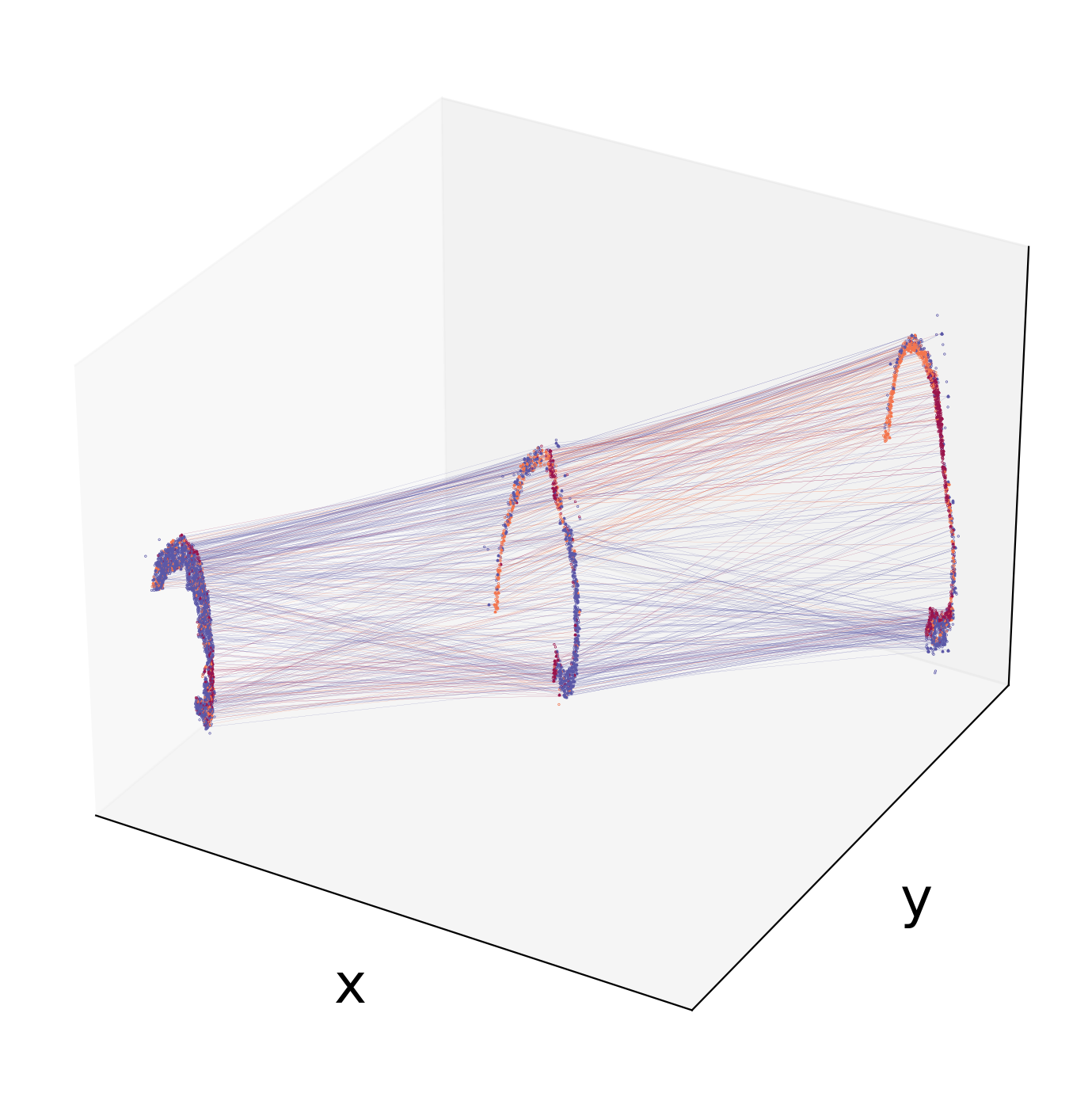
We can visualize the three sections and the line cells with the maximum transition probability in a 3D space.
[13]:
spt.visual_3D_mapping_3(df_concat,df_mapping_cell,point_size=0.8,line_width=0.06,cell_color_list=['#9A154C', '#F3754E', '#5B58A7'])
We can visualize specific two consecutive sections after calculating the transition probability across the sections. Now,we can obtain the file containing cell transition probability between section 1(adata1_sub) and section 2(adata2_sub).
[14]:
pi_df=spt.map_data(pi12,adata1_sub,adata2_sub)
Before visualizing, users are given the option to retain higher values of the maximum transition probability values based on their distribution.
[15]:
# import seaborn as sns
# sns.displot(pi_df['pi_value'],bins=200)
# pi_df_new=pi_df.loc[pi_df['pi_value']>cutoff_value]
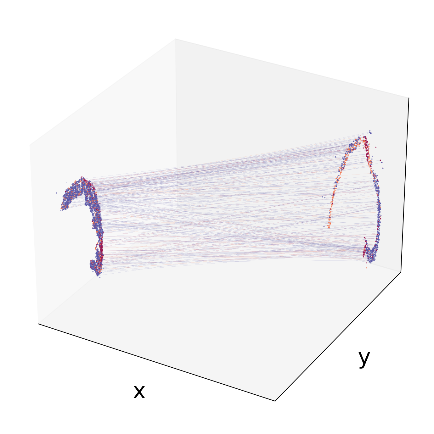
Visualize cell transfer between two sections by 3D
[16]:
spt.visual_3D_mapping_2(df_concat,pi_df[['slice1','slice2']],point_size=1,line_width=0.05,cell_color_list=['#9A154C', '#F3754E', '#5B58A7'])
5.Construct gene regulation network
Here, we use adata from E12.5 and E14.5 as an example to construct regulatory network between TF genes and target genes inferred along the developmental trajectory between two time points.TF genes list of Mouse and Human can be download from the link.
[17]:
adata1_sub.write('./E12.5.adata.h5ad')
adata2_sub.write('./E14.5.adata.h5ad')
[18]:
pi_df=spt.map_data(pi12,adata1_sub,adata2_sub)
pi_df.to_csv('./cell_mapping.csv')
[19]:
gr = spt.Trainer(
data_type='2_time',
expression_matrix_path=['./E12.5.adata.h5ad','./E14.5.adata.h5ad'],
cell_mapping_path='./cell_mapping.csv',
tfs_path='../../../../data/mouse.midbrain.three.time/ms.TF.tsv',
min_cells=[50,20], #recommend maintaining gene expression in ~ 3% of cells.
cell_generate_per_time=10000,
cell_select_per_time=50
)
gr.run(training_times=10,iter_times=30)
Train 10: 100%|██████████| 300/300 [02:37<00:00, 1.90it/s, train_loss=0.0144, test_loss=0.0158]
Weight relationships of tfs and genes are stored in weights.csv.
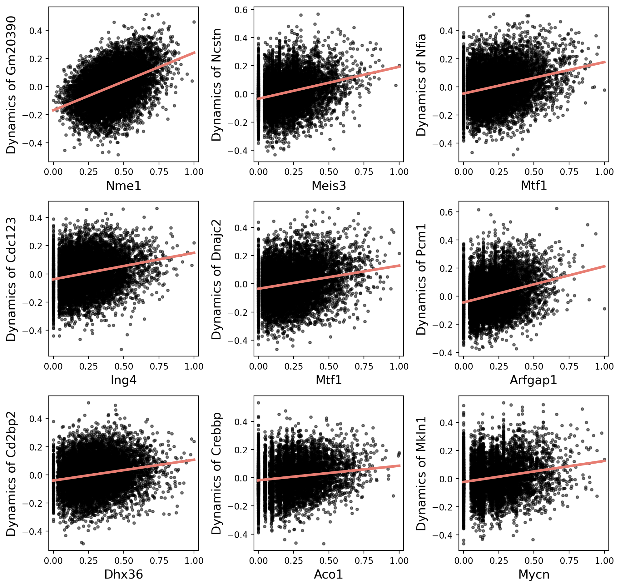
Show the relationship between TF and target genes by scatter diagram.
[20]:
gr.plot_scatter()
Get weights between TFs and genes.
[21]:
gr.network_df
[21]:
| TF | gene | weight | |
|---|---|---|---|
| 347 | Nme1 | Gm20390 | 0.031272 |
| 950 | Meis3 | Ncstn | 0.021513 |
| 1197 | Mtf1 | Nfia | 0.021020 |
| 2294 | Ing4 | Cdc123 | 0.020342 |
| 1785 | Mtf1 | Dnajc2 | 0.020236 |
| ... | ... | ... | ... |
| 1630 | Chd1 | Foxk2 | 0.010869 |
| 435 | Creb1 | Cnot8 | 0.010869 |
| 2862 | Chd1 | Kdm2a | 0.010868 |
| 694 | Srebf1 | Vps4b | 0.010868 |
| 284 | Apex1 | Ostc | 0.010867 |
3000 rows × 3 columns
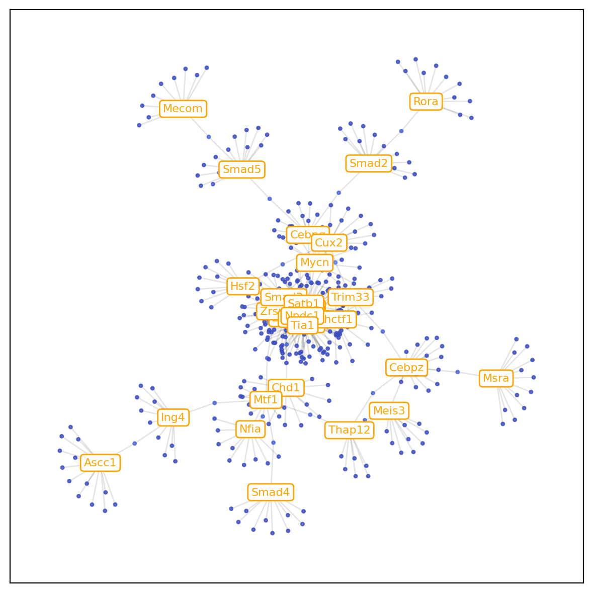
Plot the gene regulatory network diagram according to the 'gr.network_df'.
[22]:
gr.plot_gene_regulation(min_weight=0.012,min_node_num=10)
num of weight pairs after weight filtering: 1388
num of weight pairs after node_count filtering: 394