Apply spaTrack on spatial data of Intrahepatic cholangiocarcinoma cancer

Rebuilding lineages of tumorigenesis can improve us understand the deterioration and developmental process of primary tumors and describe the behaviors of malignant cells.Considering the heterozygosity and complex of malignant cells, it is possible that tumors originate from multiple starte regions. Here, we performed spaTrack to rebuild the diverse lineages of ICC tumorigenesis by spatial transcriptomics data of ICC tumor section. This notebook uses the intrahepatic cholangiocarcinoma cancer (ICC) ST data to show how spaTrack infer trajectories when data has multiple origins. Spatial transcriptomics data of ICC can be download from Baidu Netdisk and Google Drive.

import warnings

warnings.filterwarnings("ignore")

import spaTrack as spt
import scanpy as sc
import pandas as pd
import numpy as np
import matplotlib.pyplot as plt

sc.settings.verbosity = 0
plt.rcParams['figure.dpi'] = 200 #分辨率

1. Prepare ICC adata

Convert tsv files to scanpy adata (the tsv file format was described in 01 notebook).

adata = sc.read("../../../../data/ICC.ST.data/ICC.primary.ST.exp_count.tsv", cache=True)
anno = pd.read_table("../../../../data/ICC.ST.data/ICC.primary.ST.annot.tsv")

adata.obs.index = anno["ID"].values
adata.obs["cluster"] = anno["cluster"].values
adata.obsm["X_spatial"] = anno[["x", "y"]].values
adata.layers["counts"] = adata.X

Perform basic preprocessing and visualize spatial data.

sc.pp.filter_genes(adata,min_cells=10)
sc.pp.normalize_total(adata,target_sum=1e4)
sc.pp.log1p(adata)
fig, axs = plt.subplots(figsize=(6, 9))
ax = sc.pl.embedding(adata,  basis='X_spatial', show=False, color='cluster', ax=axs, frameon=False, title=' ', palette='tab20c', size=150, legend_fontsize=20)

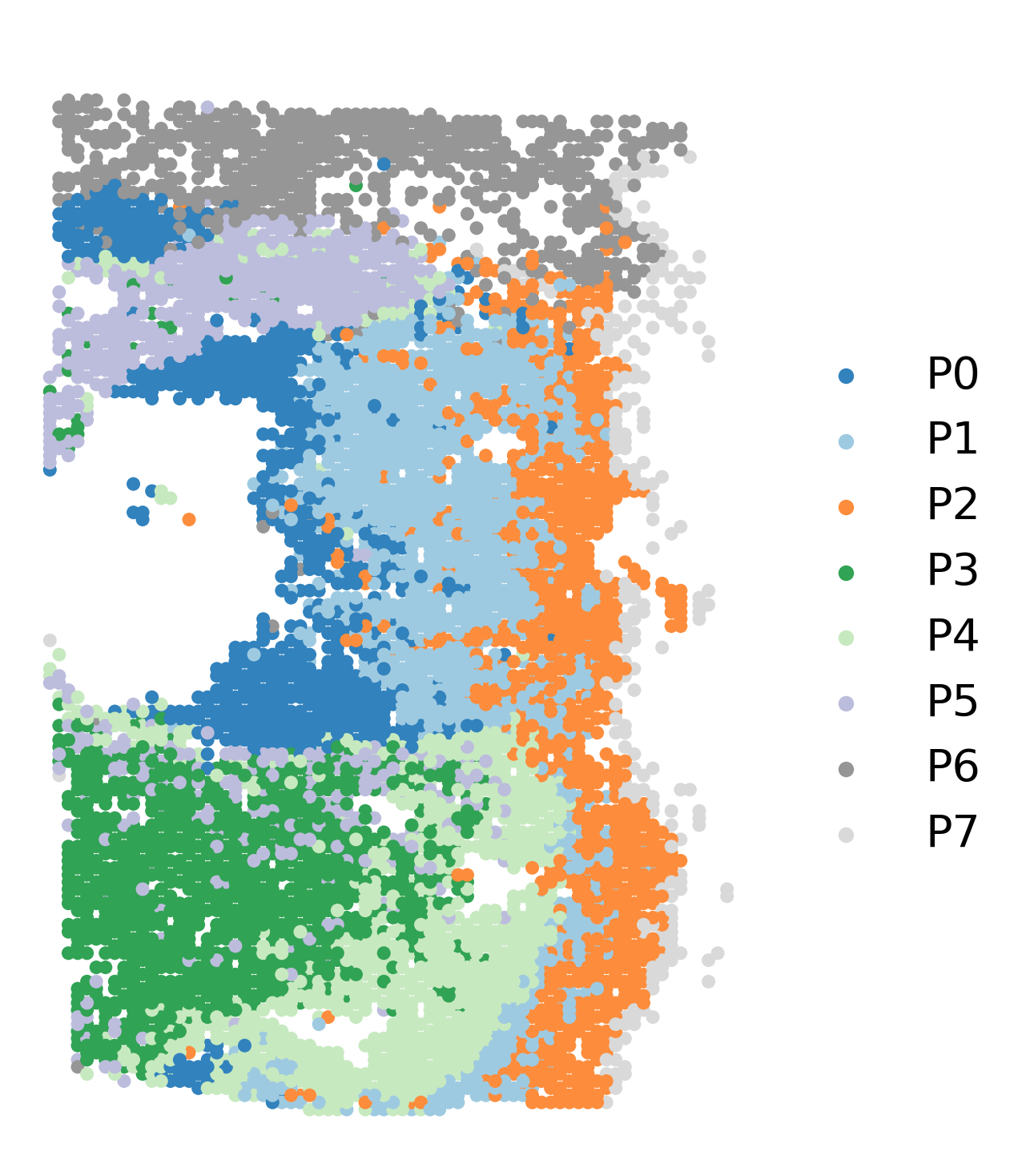
2. Choose start cells

In order to identify potential start regions, multiple factors were considered. We recommend that users manually slecte starting cluster base on prior knowledge within this field. In cases where prior knowledge and biological evidence were not available to support the selection of start cells, we suggested using entropy value.

In our analysis of the ICC tumor ST data, we found that the P0 cluster demonstrated a relatively high entropy value, indicating more likely to be starting cluster compared to the other clusters. As a result, P0 was selected as the starting cluster for further investigation.

adata = spt.assess_start_cluster(adata)

Cluster order sorted by entropy value:  ['P0', 'P1', 'P5', 'P2', 'P4', 'P3', 'P6', 'P7']

spt.assess_start_cluster_plot(adata)

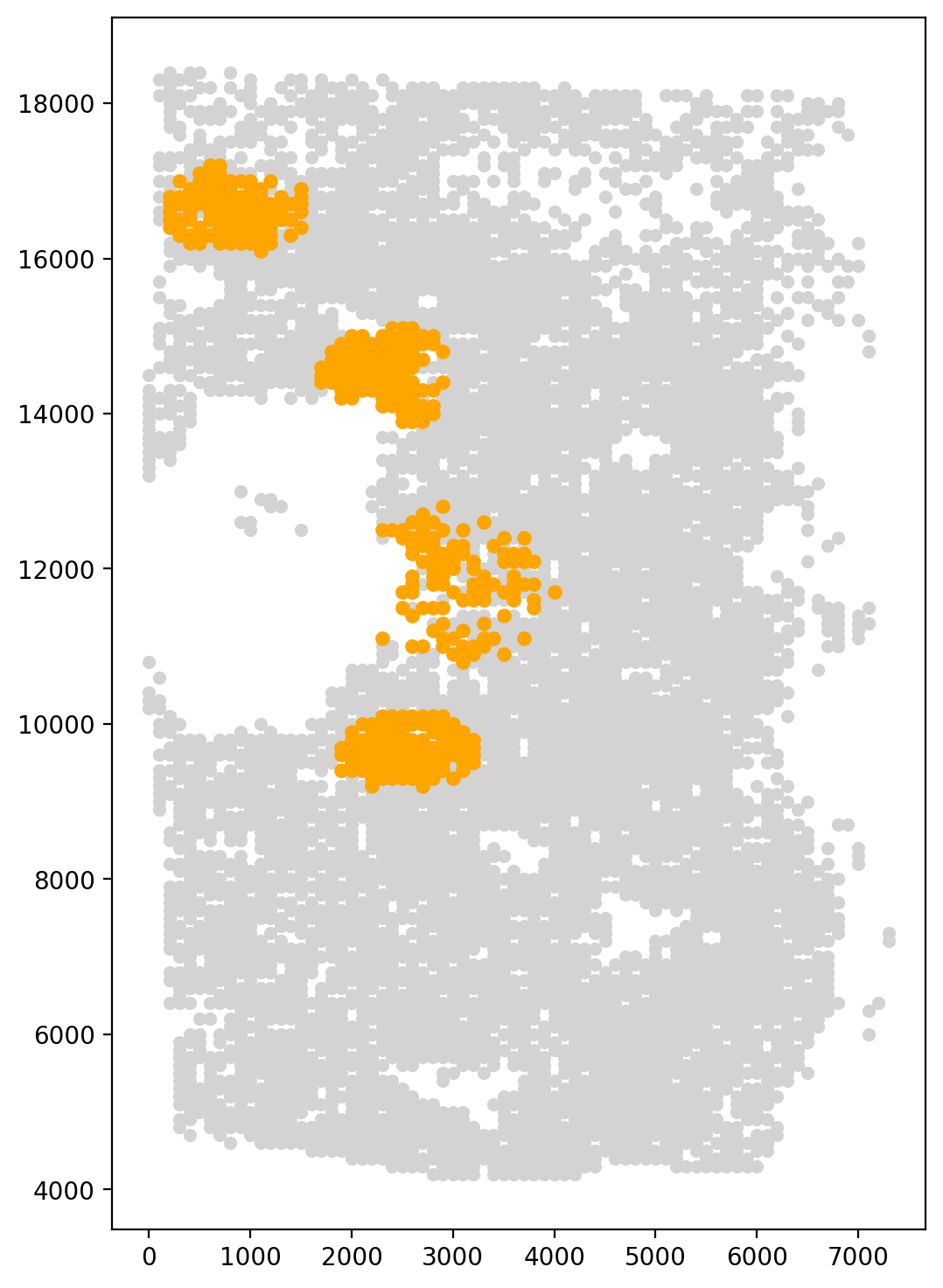
Since the P0 cluster was distributed across four distinct regions, we used the k-means method with a cluster number of 4 to identify the aggregation points of the P0 cluster. Neighbor cells were then taken as start cells for the trajectory inference.

fig, axs = plt.subplots(figsize=(6, 9))
start_cells=spt.set_start_cells(adata,select_way='cell_type',split=True,cell_type='P0',n_neigh=100,n_clusters=4)

plt.scatter(adata.obsm['X_spatial'][:,0],adata.obsm['X_spatial'][:,1],c='#D3D3D3',s=20)
plt.scatter(adata.obsm['X_spatial'][start_cells][:,0],adata.obsm['X_spatial'][start_cells][:,1],c='orange',s=25)

kmeans cluster centers:
[ 2377.98165138 14477.52293578]
[2571.73144876 9450.17667845]
[  866.37931034 16618.10344828]
[ 3020.42253521 11792.25352113]

<matplotlib.collections.PathCollection at 0x7f44939f41c0>

3. Calculate cell transition probability

Parameter estimation of alpah1 for gene expression and alpah2 for spatial distance. Calculate cell transition probability based on gene expression matrix and cell spatial coordinate.

adata.obsp['trans']=spt.get_ot_matrix(adata,data_type='spatial',alpha1=0.587,alpha2=0.413)

X_pca is not in adata.obsm, automatically do PCA first.
alpha1(gene expression): 0.587   alpha2(spatial information): 0.413

4. Caculate cell pseudotime

Assign a pseudo-time value to each cell.

adata.obs['ptime']=spt.get_ptime(adata,start_cells)

5. Calculate vector field velocity.

Calculate vector field velocity by averaging the velocities of each cell and its neighbors.

adata.uns['E_grid'],adata.uns['V_grid']=spt.get_velocity(adata,basis='spatial',n_neigh_pos=100)

The velocity of cells store in 'velocity_spatial'.

6. Plot results

Visualization of cell pseudotime and inferred cell trajectory.

fig, axs = plt.subplots(ncols=2, nrows=1, figsize=(9, 6))

sc.pl.embedding(adata, basis='X_spatial', color='ptime', show=False, ax=axs[0], color_map='Reds', title='Ptime',size=120)
vf_velocity = sc.pl.embedding(adata, basis='X_spatial', show=False, ax=axs[1],color='cluster', legend_loc=None, frameon=False, title='Trajectory', alpha=0.6, size=120)
vf_velocity.streamplot(adata.uns['E_grid'][0], adata.uns['E_grid'][1], adata.uns['V_grid'][0], adata.uns['V_grid'][1], color='black', linewidth=2,density=1.2,arrowsize=1.2)

<matplotlib.streamplot.StreamplotSet at 0x7f448c05d850>

7. Downstream analysis

In order to apply the LAP algorithm to spatial transcriptomics data, we need to reconstruct the grid-level vector field into cell-level data. This is done by interpolating the vector field values from the grid points to the cell locations, which enables us to calculate the velocity vectors for individual cells. The cell-level vector field is then used as input to the LAP algorithm to infer the optimal transition path between the chosen start and end points.

VecFld = spt.VectorField(adata, basis="spatial")

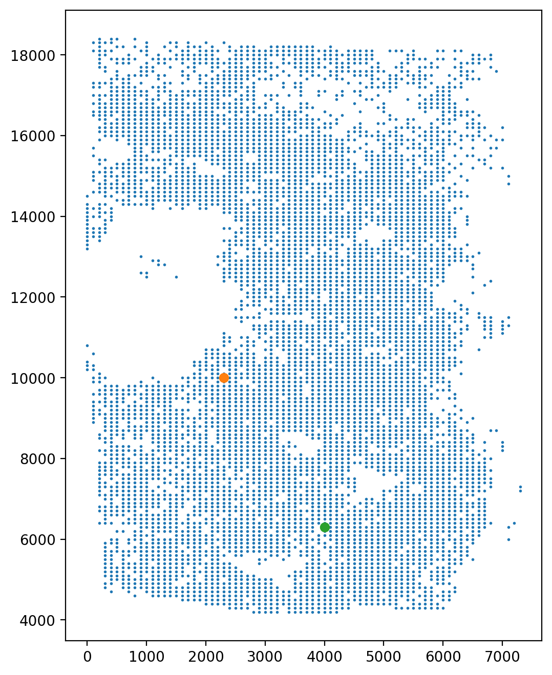
7.1 Least Action Path (LAP)

Select the start point and the end point across the direction of trajectory.

fig, axs = plt.subplots(ncols=1, nrows=1, figsize=(6, 8))

LAP_start_point = [2300, 10000]
LAP_end_point = [4000, 6300]
LAP_start_cell = spt.nearest_neighbors(LAP_start_point, adata.obsm["X_spatial"])[0][0]
LAP_end_cell = spt.nearest_neighbors(LAP_end_point, adata.obsm["X_spatial"])[0][0]

plt.scatter(*adata.obsm["X_spatial"].T, s=1)
plt.scatter(*adata[LAP_start_cell].obsm["X_spatial"].T)
plt.scatter(*adata[LAP_end_cell].obsm["X_spatial"].T)

<matplotlib.collections.PathCollection at 0x7f4464e3d5b0>

Get the neighbors according to the spatial location.

sc.pp.neighbors(adata, use_rep="X_spatial", key_added="X_spatial", n_neighbors=100)

Calculate the least action path between given start cell and end cell.

lap = spt.least_action(
    adata,
    init_cells=adata.obs_names[LAP_start_cell],
    target_cells=adata.obs_names[LAP_end_cell],
    vecfld=VecFld,
    basis="spatial",
    adj_key="X_spatial_distances",
    EM_steps=5,
    n_points=20,
)

Visualization of LAP and color bar represents pseudotime.

LAP_ptime,LAP_nbrs=spt.lap.map_cell_to_LAP(adata)
sub_adata=adata[LAP_nbrs,:]
sub_adata.obs['ptime']=LAP_ptime
sub_adata=sub_adata[np.argsort(sub_adata.obs["ptime"].values), :].copy()

fig, ax = plt.subplots(figsize=(6,8))
plt.axis('off')
ax = sc.pl.embedding(adata,  basis='X_spatial',color='cluster',show=False,ax=ax,frameon=False,legend_loc=None,alpha=0.4,size=150)
ax.streamplot(adata.uns['E_grid'][0], adata.uns['E_grid'][1], adata.uns['V_grid'][0], adata.uns['V_grid'][1],density=1.2,color='black',linewidth=2.5,arrowsize=1.5,minlength=0.1,maxlength=0.8)
ax = spt.plot_least_action_path(adata,basis='spatial',ax=ax,point_size=120,linewidth=5)
sc.pl.embedding(sub_adata, basis='X_spatial',ax=ax, color="ptime", cmap="Purples",frameon=True,size=150,title=' ')

7.2 Pseudotime-dependent genes on LAP

Choose cell type of interest on LAP and filter genes with high variability which larger than minimum expression proportion.

sub_adata_path = sub_adata[sub_adata.obs["cluster"].isin(["P0", "P3", "P4"])]
sub_adata_path = spt.filter_gene(sub_adata_path, min_exp_prop=0.1, hvg_gene=5000)

clusters ordered by ptime:  ['P0', 'P3', 'P4']
Cell number     594
Gene number     1268

To investigate the relationship between gene expression changes and pseudotime values, we applied the generalized additive model (GAM). This allowed us to filter for pseudotime-dependent genes based on their model fit (R2) and false discovery rate (FDR). Only genes that showed significant associations with pseudotime values were selected as pseudotime-dependent genes.

df_res  = spt.ptime_gene_GAM(sub_adata_path,core_number=5)

Genes number fitted by GAM model:   1268

df_sig_res = df_res.loc[(df_res['model_fit']>0.15) & (df_res['fdr']<0.05)]
sort_exp_sig = spt.order_trajectory_genes(sub_adata_path,df_sig_res,cell_number=20)

Finally selected 54 genes.

Use heatmap to display pseudotime-dependent genes.

spt.plot_trajectory_gene_heatmap(sort_exp_sig,smooth_length=100,gene_label_size=15,cmap_name='twilight_shifted')

Show example of pseudotime-dependent genes.

spt.plot_trajectory_gene(sub_adata_path,gene_name='AQP1')

<Axes: title={'center': 'AQP1'}, xlabel='ptime', ylabel='expression'>

spt.plot_trajectory_gene(sub_adata_path,gene_name='ITGA3')

<Axes: title={'center': 'ITGA3'}, xlabel='ptime', ylabel='expression'>